Chapter 3 Wednesday: Competing risk
3.1 Key (operative) concepts
Patient are exposed simultaneously to \(k (\geq2)\) causes
Effect Free Survival (EFS) is univariate, i.e. only the First Observed Event (FOE) is considered and of interest
The interest is not in the survival model
“At \(\infty\) all individuals will not die in the ICU”
- Type of observed time
- Cansored (conventionally coded w/ \(0\))
- Failure w/ a FOE different from the last absorbing one (coded w/ \(1 -- k-1\))
- Failure w/ the FOE as the last absorbing event (coded w/ \(k\))
- \(T_k = min\Bigl(\tilde{T_k}^{D_k} | D_k \in \{\textrm{causes of failure for }k\} \Bigr)\)
Cumulative Incidence Function (CIF) do not require independence between causes
In competing risk, K-M is biased, i.e. overestimates the CIF (because it the independence assumption is violated)
- Tests
- w/out competing risk: log-rank
- w/ competing risk: modified \(\chi^2\) (Gray 1988)
- Regression strategies for competing risk
- Case Specific Hazard Ratio (CS-HR) — Cox, useful for clinical interests (present it for each competing risk taken singularly)
- Subdistribution Hazard Ratio (SHR) — Fine-Gray, useful for administrative] interests (present it for the global risk considering the contribution of each competing one)
Test the proportional hazard assumption for SHR
There are formulas for the sample size calculation when considering competing risk
3.2 Data manipulation
set.seed(171004)
data(mgus, package = 'survival')
# ?mgus

mgus_df <- as_tibble(mgus)
dd <- datadist(mgus_df)

mgus_df
## # A tibble: 241 x 12
## id age sex dxyr pcdx pctime futime death alb creat hgb
## * <dbl> <dbl> <fctr> <dbl> <fctr> <dbl> <dbl> <dbl> <dbl> <dbl> <dbl>
## 1 1 78 female 68 <NA> NA 748 1 2.8 1.2 11.5
## 2 2 73 female 66 LP 1310 6751 1 NA NA NA
## 3 3 87 male 68 <NA> NA 277 1 2.2 1.1 11.2
## 4 4 86 male 69 <NA> NA 1815 1 2.8 1.3 15.3
## 5 5 74 female 68 <NA> NA 2587 1 3.0 0.8 9.8
## 6 6 81 male 68 <NA> NA 563 1 2.9 0.9 11.5
## 7 7 72 female 68 <NA> NA 1135 1 3.0 0.8 13.5
## 8 8 79 female 69 <NA> NA 2016 1 3.1 0.8 15.5
## 9 9 85 female 70 <NA> NA 2422 1 3.2 1.0 12.4
## 10 10 58 male 65 <NA> NA 6155 1 3.5 1.0 14.8
## # ... with 231 more rows, and 1 more variables: mspike <dbl>- Find number of patient w/ malignancy (AKA transition), death (w/out malignancy) and Free of Events.
mgus_df <- mgus_df %>%
  mutate(
    malignancy = !is.na(pcdx)
  )

mgus_df %>%
  group_by(malignancy, death) %>%
  summarise(n = n())
## # A tibble: 4 x 3
## # Groups: malignancy [?]
## malignancy death n
## <lgl> <dbl> <int>
## 1 FALSE 0 14
## 2 FALSE 1 163
## 3 TRUE 0 2
## 4 TRUE 1 62Patients w/ malignancy as a FOE are 64; patients which experiment death as FOE are 163, while the ones FoE are 14. 163.
- Find the indicator for censored, malignancy and death (
indicator) - Find the time-to-event to use in the models (
time_t)
mgus_df <- mgus_df %>%
  mutate(
    indicator = if_else(malignancy, 1, 2 * death),
    time_t    = pmin(futime, pctime, na.rm = TRUE)
)

mgus_df
## # A tibble: 241 x 15
## id age sex dxyr pcdx pctime futime death alb creat hgb
## <dbl> <dbl> <fctr> <dbl> <fctr> <dbl> <dbl> <dbl> <dbl> <dbl> <dbl>
## 1 1 78 female 68 <NA> NA 748 1 2.8 1.2 11.5
## 2 2 73 female 66 LP 1310 6751 1 NA NA NA
## 3 3 87 male 68 <NA> NA 277 1 2.2 1.1 11.2
## 4 4 86 male 69 <NA> NA 1815 1 2.8 1.3 15.3
## 5 5 74 female 68 <NA> NA 2587 1 3.0 0.8 9.8
## 6 6 81 male 68 <NA> NA 563 1 2.9 0.9 11.5
## 7 7 72 female 68 <NA> NA 1135 1 3.0 0.8 13.5
## 8 8 79 female 69 <NA> NA 2016 1 3.1 0.8 15.5
## 9 9 85 female 70 <NA> NA 2422 1 3.2 1.0 12.4
## 10 10 58 male 65 <NA> NA 6155 1 3.5 1.0 14.8
## # ... with 231 more rows, and 4 more variables: mspike <dbl>,
## # malignancy <lgl>, indicator <dbl>, time_t <dbl>- Estimate the naive K-M and the cumulative incidence functions
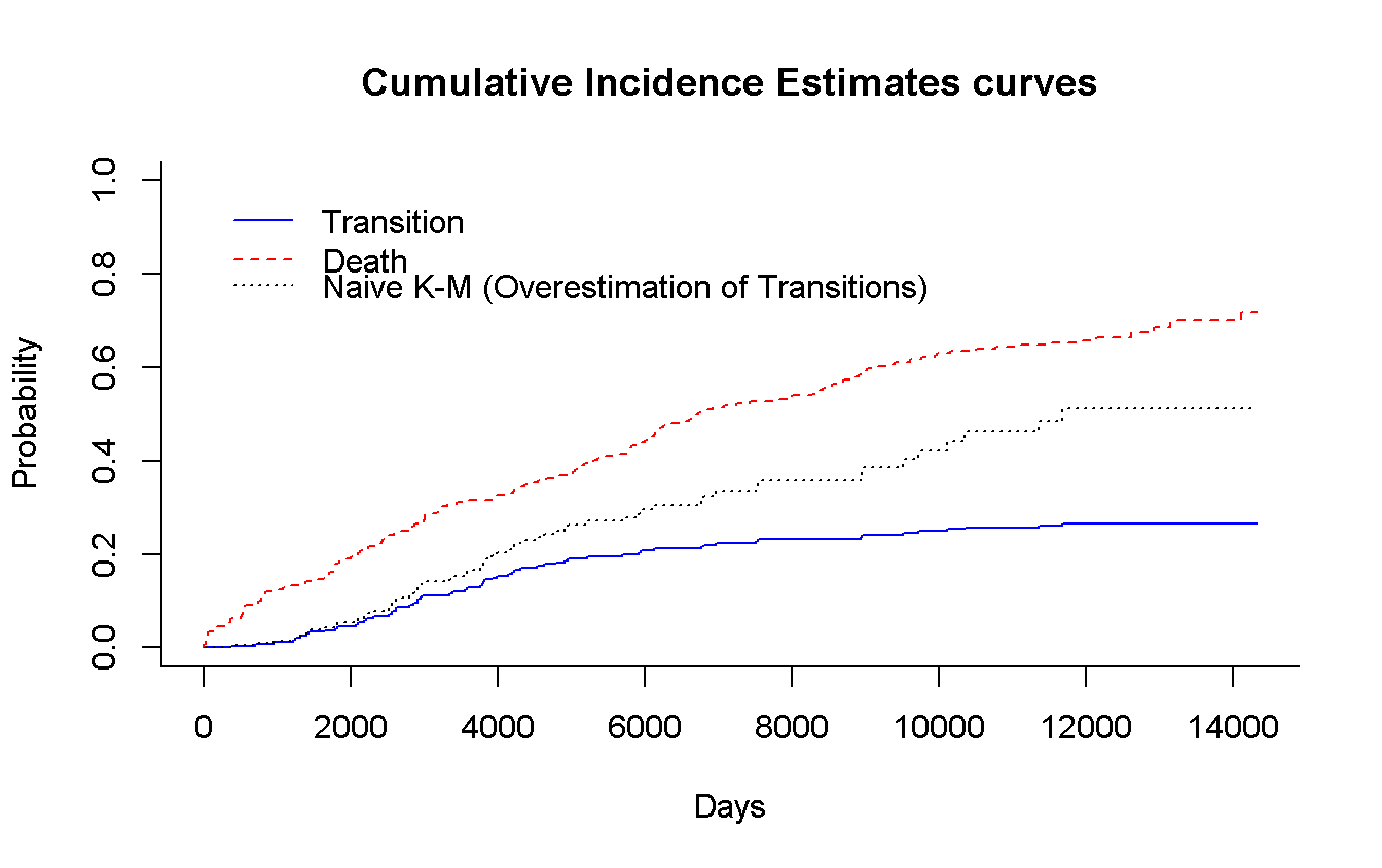
# Using survival
cuminc(mgus_df$time_t, mgus_df$indicator) %>%                  # ?cmprsk::cuminc
  plot(                                                  # ?cmprsk:::plot.cuminc
    main    = 'Cumulative Incidence Estimates curves',
    col     = c('blue', 'red'),
    xlab    = 'Days',
    curvlab = c('Transition', 'Death'),
    wh      = c(1, 1)                                          # legend position
)

survfit(Surv(time_t, malignancy) ~ 1,        # using `rms::npsurv()` is the same
  data = mgus_df
  ) %>%
  lines(                          # Use `lines()` to draw over the previous plot
    fun       = 'event',                            # plot the cumulative events
    conf.int   = FALSE,
    col       = 'black',
    lty       = 3
)
legend(x = 1, y = 0.86,
  legend = 'Naive K-M (Overestimation of Transitions)',
  col    = 'black',
  lty    = 3,
  bty    = 'n' # remove box arround the legend (because we have to add an entry)
)
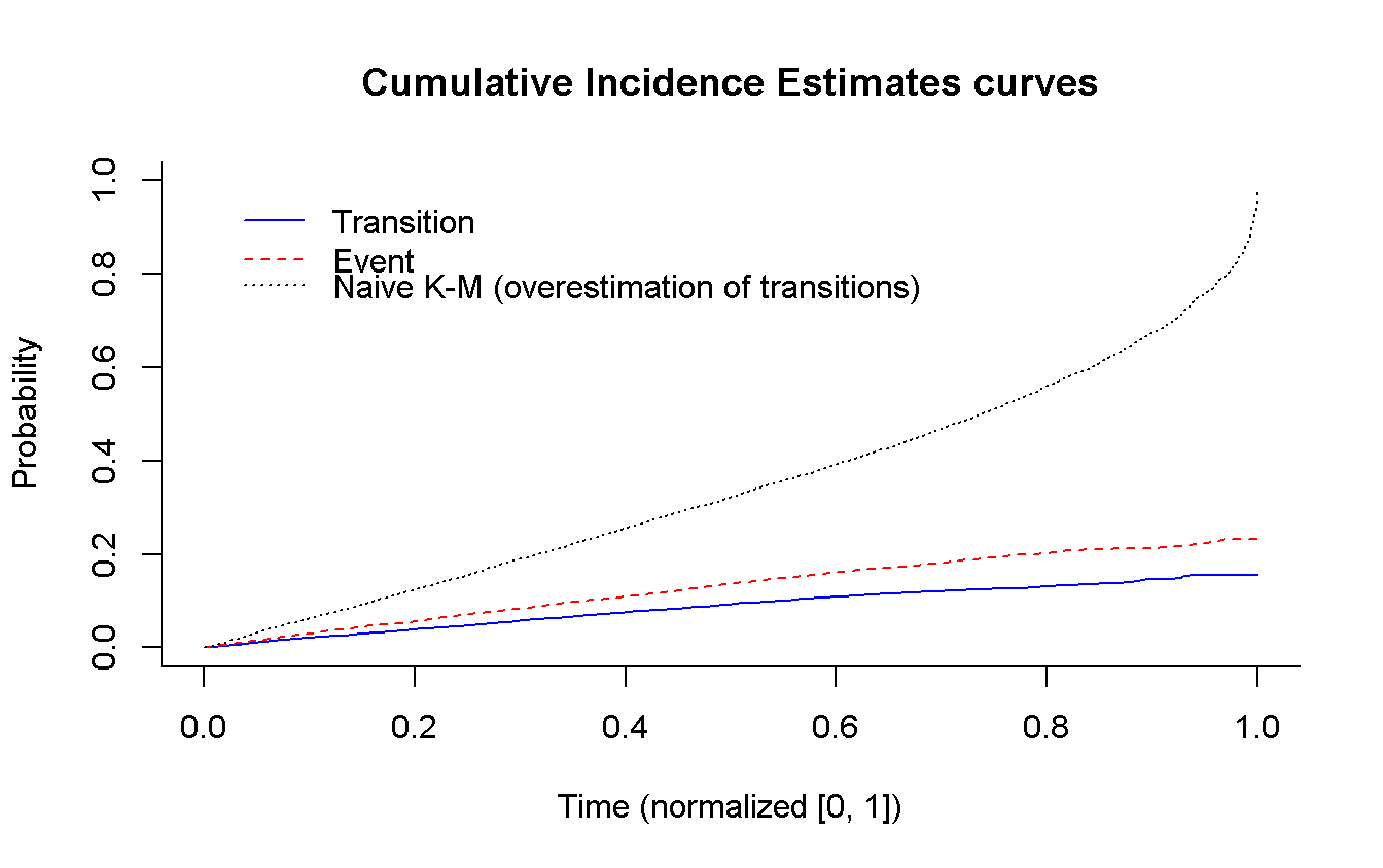
3.3 Simulation of Competing risk
- Specify two cause-specific exponential hazard \(\lambda_1(t)\) and \(\lambda_2(t)\) of means \(0.8\) and \(1.2\). (Set sample size as you like.)
n        <- 1e4
lambda_1 <- 0.8
lambda_2 <- 1.2- Simulate survival times \(T\) based on the all causes hazard \(\lambda_.(t) = \lambda_1(t) + \lambda_2(t)\).
lambda    <- lambda_1 + lambda_2
surv_time <- rexp(n,
  rate = 1 / lambda
)- Generate Bernoulli \(B(p)\) random variables, w/ \(p = \lambda_1(t) / \lambda_.(t)\), i.e. is the probability of occurrence of the event of type 1.
p_cens     <- lambda_1 / lambda
transition <- rbinom(n,
  size = 1,
  prob = p_cens
) %>%
as.logical # Set as logical to use the variable for conditional statements- Simulate uniform censoring times over \([0, 1]\).
censor_time <- runif(n,
  min = 0,
  max = 1
)- Estimate the Cumulative Incidence of each competing event, w/ and w/out censoring; discuss the results.
# create the dataset
sim_data <- data_frame(
  id         = seq_len(n),
  transition = transition,
  surv_t     = surv_time,
  cens_t     = censor_time,
  time_t     = pmin(surv_t, cens_t),
  status     = case_when(
    time_t == cens_t ~ 0L,              # All the censored patients has status 0
    transition       ~ 1L,    # Among the other, the ones which has a transition
                              # have state 1
    TRUE             ~ 2L     # All the other were dead (before the end of f-up)
  )
)

# Explore a (random) sample of three cases for each staus
sim_data %>%
  group_by(status) %>%
  sample_n(3)
## # A tibble: 9 x 6
## # Groups: status [3]
## id transition surv_t cens_t time_t status
## <int> <lgl> <dbl> <dbl> <dbl> <int>
## 1 6759 FALSE 6.844765752 0.5175084 0.517508388 0
## 2 906 TRUE 1.378642827 0.5063402 0.506340163 0
## 3 3568 TRUE 0.623047318 0.5752797 0.575279657 0
## 4 2196 TRUE 0.506380841 0.9344626 0.506380841 1
## 5 8119 TRUE 0.157231928 0.9007847 0.157231928 1
## 6 5854 TRUE 0.742379822 0.8771130 0.742379822 1
## 7 1685 FALSE 0.539729742 0.9635529 0.539729742 2
## 8 4550 FALSE 0.001042022 0.3692372 0.001042022 2
## 9 6893 FALSE 0.410360153 0.9322769 0.410360153 2# Using survival
cuminc(sim_data$time_t, sim_data$status) %>% # ?cmprsk::cuminc
plot( # ?cmprsk:::plot.cuminc
main = 'Cumulative Incidence Estimates curves',
col = c('blue', 'red'),
xlab = 'Time (normalized [0, 1])',
curvlab = c('Transition', 'Event'),
wh = c(0.01, 1) # legend position
)
survfit(Surv(time_t, transition) ~ 1, # using `rms::npsurv()` is the same
data = sim_data
) %>%
lines( # Use `lines()` to draw over the previous plot
fun = 'event', # plot the cumulative events
conf.int = FALSE,
col = 'black',
lty = 3
)
legend(x = 0.01, y = 0.86,
legend = 'Naive K-M (overestimation of transitions)',
col = 'black',
lty = 3,
bty = 'n' # remove box arround the legend (because we have to add an entry)
)
3.4 Estimation of the effect of sex on MGUS incidence
- Compare the results of Cox cause specific hazard model…
For clinical questions, i.e. cause specific risk to experiment the event w/out taking into account the other couse(s)
dd <- datadist(mgus_df)

cox_sex <- cph(Surv(time_t, malignancy) ~ sex,
  data = mgus_df,
  x    = TRUE,
  y    = TRUE
)

summary(cox_sex)                  # this is good for a clean view of the effects
## Effects Response : Surv(time_t, malignancy)
##
## Factor Low High Diff. Effect S.E. Lower 0.95 Upper 0.95
## sex - female:male 2 1 NA 0.049342 0.25103 -0.44268 0.54136
## Hazard Ratio 2 1 NA 1.050600 NA 0.64232 1.71830cox_sex # Here there are more informations (and the p-values)## Cox Proportional Hazards Model
##
## cph(formula = Surv(time_t, malignancy) ~ sex, data = mgus_df,
## x = TRUE, y = TRUE)
##
## Model Tests Discrimination
## Indexes
## Obs 241 LR chi2 0.04 R2 0.000
## Events 64 d.f. 1 Dxy -0.039
## Center -0.028 Pr(> chi2) 0.8441 g 0.024
## Score chi2 0.04 gr 1.025
## Pr(> chi2) 0.8441
##
## Coef S.E. Wald Z Pr(>|Z|)
## sex=male -0.0493 0.2510 -0.20 0.8442
## Predict(cox_sex) %>% # It is necessary to have the predictions for the plot
plot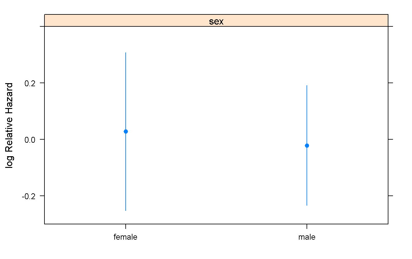
cox_sex_death <- cph(Surv(time_t, indicator == 2) ~ sex,
  data = mgus_df,
  x    = TRUE,
  y    = TRUE
)

summary(cox_sex_death)
## Effects Response : Surv(time_t, indicator == 2)
##
## Factor Low High Diff. Effect S.E. Lower 0.95 Upper 0.95
## sex - female:male 2 1 NA -0.44221 0.16183 -0.75939 -0.12502
## Hazard Ratio 2 1 NA 0.64262 NA 0.46795 0.88248cox_sex_death## Cox Proportional Hazards Model
##
## cph(formula = Surv(time_t, indicator == 2) ~ sex, data = mgus_df,
## x = TRUE, y = TRUE)
##
## Model Tests Discrimination
## Indexes
## Obs 241 LR chi2 7.65 R2 0.031
## Events 163 d.f. 1 Dxy 0.124
## Center 0.2514 Pr(> chi2) 0.0057 g 0.218
## Score chi2 7.59 gr 1.243
## Pr(> chi2) 0.0059
##
## Coef S.E. Wald Z Pr(>|Z|)
## sex=male 0.4422 0.1618 2.73 0.0063
## Predict(cox_sex_death) %>%
plot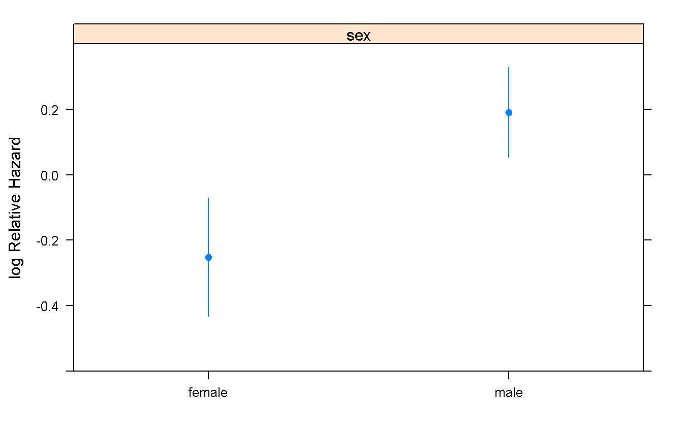
- …to those of the Fine and Gray model
For administrative questions, i.e. overall risk of experiment each event taking into account the competing risk
mgus_num <- mgus_df %>%
  mutate(sex = as.numeric(sex))

crr(                                      # We do not have a plot method for crr
  ftime   = mgus_num$time_t,
  fstatus = mgus_num$indicator,
  cov1    = mgus_num$sex
) %>%
  summary
## Competing Risks Regression
##
## Call:
## crr(ftime = mgus_num$time_t, fstatus = mgus_num$indicator, cov1 = mgus_num$sex)
##
## coef exp(coef) se(coef) z p-value
## mgus_num$sex1 -0.339 0.713 0.249 -1.36 0.17
##
## exp(coef) exp(-coef) 2.5% 97.5%
## mgus_num$sex1 0.713 1.4 0.437 1.16
##
## Num. cases = 241
## Pseudo Log-likelihood = -341
## Pseudo likelihood ratio test = 1.83 on 1 df,References
Gray, Robert J. 1988. “A Class of K-Sample Tests for Comparing the Cumulative Incidence of a Competing Risk.” The Annals of Statistics. JSTOR, 1141–54.